
Introduction
This is an example taken from Invariant Risk Minimization, Appendix D. I've taken that basic code and expanded upon it with some plots and narration of what's going on. I won't provide a full exposition of the method here, but only some notes which I hope may be a helpful supplement to anyone trying to use the code. For full details I encourage you to read the paper, which is very well written and features a charming Socratic dialogue at the end! It's probably one of my favorite papers from recent years.
The full code to reproduce the paper can also be found on GitHub. You can find this notebook and run it yourself on Google Colab.
Imports
import numpy as np
import matplotlib.pyplot as plt
%matplotlib inline

import torch
from torch import nn, optim
Motivation and Data Generation
In IRM we use the concept of environments. We presume the data is being pulled from different environments which have different data distributions, and we don't know at test time what environment we will be seeing data from. So we want to generalize across all potential environments (including those not seen at train time).
So the training data consists of multiple "environments", and the training algorithm uses this knowledge to avoid learning correlations that do not persist across all environments.
In our case, different environments will simply amount to a different variance on the distribution the data is sampled from. Repeating Example 1 from the IRM paper, here is our data generation process:
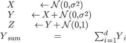
The trick here is we will try to learn a function $f(X, Z) \rightarrow Y_{sum}$. Oh no! Part of our input ($Z$) actually depends on our output, $Y$! So the true structural equation model actually looks like $X \rightarrow Y \rightarrow Z$.
Below, we'll generate a number of different environments using different values of $\sigma$. Each environment will be equally represented (they will have the same number of samples), but some environments will exist only in the test set, and not in the training set. We will see that this will cause problems.
def example_1(n=10000, dim=2, sigma=1):
    """
    Generate data of the form from Example 1 of the paper:
      - X <- N(0, sigma^2)
      - Y <- X + N(0, sigma^2)
      - Z <- Y + N(0, 1)
      - Y_sum <- sum(Y)

    :param n: Number of data points.
    :param dim: Dimensionality of the data points.
    :param sigma: The standard deviation of the noise distribution.
    :returns: tuple(tensor(X, Z), tensor(Y_sum))
    """
    x = torch.randn(n, dim) * sigma
    y = x + torch.randn(n, dim) * sigma
    z = y + torch.randn(n, dim)
    return torch.cat((x, z), 1), y.sum(1, keepdim=True)

# Sample training data with one low variance and one high variance.
train_sigmas = (0.1, 1.0)
train_environments = [example_1(sigma=s) for s in train_sigmas]
# Sample testing data with the same sigmas, but also more in between.
test_sigmas = (0.01, 0.1, 1.0)
test_environments = [example_1(sigma=s) for s in test_sigmas]
Visualize the data.
for envname, environments in zip(("Train", "Test"), (train_environments, test_environments)):
    for i, (x_e, y_e) in enumerate(environments):
        fig = plt.figure(figsize=(15, 2))
        fig.suptitle(f"{envname} Environment {i+1}")
        num_variables = x_e.shape[1] + y_e.shape[1]
        plotdex = 1
        plt.subplots_adjust(top=0.7)
        for name, data in (("X", x_e), ("Y", y_e)):
            for j, col in enumerate(data.T):
                plt.subplot(1, num_variables, plotdex)
                plt.title(f"{name}_{j+1}")
                plt.ylabel("Frequency")
                plt.xlabel("Value")
                plt.hist(col, bins=50)
                plt.axis((-6, 6, 0, 700))
                plotdex += 1


Different Environments
In the plot above, each row is a different environment. Some of the test environments have similar data distributions to those in the training set. However, Test Environment 1 is drawn from a significantly different distribution than what we trained on. We see that Test Environment 3 has a strong correlation with the second two variables ($Z_1$ and $Z_2$, a.k.a. X_3 and X_4), while this correlation is thoroughly destroyed in Test Environment 1:
from scipy.stats import pearsonr

def correlation_with_input(input_x, target_y):
    return np.array([pearsonr(col, target_y.squeeze())[0] for col in input_x.T])

for i, (x_e, y_e) in enumerate(test_environments):
    print(f"Test Environment {i+1} Correlations: {correlation_with_input(x_e, y_e)}")
In general, we'd like our model to perform similarly well in all environments, so that we don't get any unpleasant surprises when we deploy it in the real world. So we want our training performance (or really, our performance on the validation set) to be predictive of our performance on the test set (a.k.a. the real world).
The IRM Penalty
The fact that we'd like our model to perform similarly on different environments is the key motivation behind IRM. Thus, the "true" IRM model is the solution to a constrained optimization problem,

The constraint we would like to impose on our data representation $\Phi$ is that the optimal classifier (or regressor) $w$ is the same in all environments. This can only be true if our representation is built only from variables whose distributions do not change across environments. So this could be a way to automatically find the invariant correlations.
However, this optimization problem is not computationally practical to solve, so Arjovsky et al. propose a relaxation of the problem where the constraint is expressed as a penalty instead:

Check out the full details in the paper. What follows is the PyTorch implementation of that penalty (the gradient norm), taken from Appendix D.
from torch import autograd

def compute_penalty(losses, dummy_w):
    """
    PyTorch implementation of the IRM penalty (the gradient norm). Taken from Appendix D of the
    paper: https://arxiv.org/abs/1907.02893

    Interestingly, here we split the environment into two random groups, average them separately,
    take their gradients separately, then use these two "gradient samples" to produce the estimated
    penalty. However, in the paper's experiment on GitHub, they don't bother doing this separate
    sampling, and instead just take the gradient of the entire average loss, then square it. It's
    unclear why they're doing it this way here, since it doesn't seem to me like it would improve
    the estimate.

    Here, then, is a simplified alternative implementation:
        grad = autograd.grad(losses.mean(), dummy_w, create_graph=True)[0]
        return torch.sum(grad**2)

    See the GitHub implementation here:
    https://github.com/facebookresearch/InvariantRiskMinimization/blob/master/code/colored_mnist/main.py#L107-L111
    """
    g1 = autograd.grad(losses[0::2].mean(), dummy_w, create_graph=True)[0]
    g2 = autograd.grad(losses[1::2].mean(), dummy_w, create_graph=True)[0]
    return (g1 * g2).sum()
Training
We know from the problem setup that our output depends on the first two parameters of the input $(X_1, X_2)$ but it does not depend on the last two parameters $(Z_1, Z_2)$. When we run this, we can see that IRM very quickly learns to squash the weight on the last two parameters to almost zero.
def print_epoch_info(epoch_idx, num_epochs, phi, avg_error, penalty, collate_prints=True):
    params = phi.detach().cpu().numpy()
    with np.printoptions(precision=3):
        # Preserve the first iteration's print, otherwise overwrite.
        if epoch_idx == 0:
            prefix = "Initial performance:\n"
            suffix = "\n"
        elif collate_prints:
            prefix = "\r"
            suffix = ""
        else:
            prefix = ""
            suffix = "\n"
        ndigits = int(np.log10(num_epochs)) + 1
        print(prefix + f"Epoch {epoch_idx+1:{ndigits}d}/{num_epochs} ({epoch_idx/num_epochs:3.0%});"
              f" params = {params.transpose()[0]};" # Print on one line.
              f" MSE = {avg_error:.4f};"
              f" penalty = {penalty:.9f}", end=suffix)


MSE_LOSS = torch.nn.MSELoss(reduction="none")

def avg_loss_per_env(model, environments, loss=MSE_LOSS):
    return np.array([float(loss(model(x_e), y_e).mean()) for x_e, y_e in environments])

def eval_dataset(model, dataset_name, dataset_envs, loss=MSE_LOSS):
    env_errors = avg_loss_per_env(model, dataset_envs, loss)
    print(f"{dataset_name} errors:")
    for i, err in enumerate(env_errors):
        print(f"Environment {i+1} Error = {err}")
    print(f"Overall Average = {env_errors.mean():.4f}")

def eval_all(model, loss=MSE_LOSS):
    for name, envs in (("Train", train_environments), ("Test", test_environments)):
        eval_dataset(model, name, envs, loss)


def train(use_IRM=True, num_epochs=50000, epochs_per_eval=1000, collate_prints=True):

    # Model: y = x.dot(phi) * dummy_w
    phi = torch.nn.Parameter(torch.ones(train_environments[0][0].shape[1], 1) * 1.0)
    dummy_w = torch.nn.Parameter(torch.Tensor([1.0]))
    def model(input):
        return input @ phi * dummy_w

    # We will only learn phi.
    opt = torch.optim.SGD([phi], lr=1e-3)
    mse = torch.nn.MSELoss(reduction="none")

    for i in range(num_epochs):
        # Sum of average error in each environment.
        error = 0
        # Total IRM penalty across all environments.
        penalty = 0

        # Forward pass and loss computation.
        for x_e, y_e in train_environments:
            p = torch.randperm(len(x_e))
            error_e = mse(model(x_e[p]), y_e[p])
            penalty += compute_penalty(error_e, dummy_w)
            error += error_e.mean()

        # Print losses.
        if i % epochs_per_eval == 0:
            print_epoch_info(i,
                             num_epochs,
                             phi,
                             error / len(train_environments),
                             penalty,
                             collate_prints)

        # Backward pass.
        opt.zero_grad()
        if use_IRM:
            # NOTE: This scaling seems arbitrary and I'm not sure if the paper provides insight as
            # to how to choose this hyperparameter.
            (1e-5 * error + penalty).backward()
        else:
            error.backward()
        opt.step()

        # Do a sanity check.
        if phi.isnan().any():
            print_epoch_info(i,
                             num_epochs,
                             phi,
                             error / len(train_environments),
                             penalty,
                             collate_prints)
            print("ERROR: Optimization diverged and became NaN. Halting training.")
            return model, phi

    params = phi.detach().cpu().numpy()
    print("\n\nFinal model:")
    print(f"params = {params.transpose()[0]}")
    eval_all(model, mse)
    return model, phi
Now we can see the comparison between IRM and a standard loss function. Note that in both cases, we have knowledge of separate environments in the training data, but we have no knowledge of the test environments or what can change between all possible environments.
irm_model, irm_params = train()
standard_model, standard_params = train(use_IRM=False)
Discussion
IRM vs. Standard Learning
As we can see from the final models above, IRM performs worse on both train and test data. What's going on?? What's the point of IRM if it doesn't improve our model?!
However, if we look more closely, we can see that in certain environments IRM does better than the standard model, while in others it does worse. Our metric, an average across environments, is a little naive and doesn't show this very well, so it could be easy to miss.
When looking at the performance breakdown per environment, we can see that the environments with lower variances is where IRM does better. When there is high variance, the spurious correlation with $Z$ will help us predict the outcome better. But when there is low variance, this assumption breaks and focusing on $X$ (the true cause of $Y$) is better.
This leads to a few questions. One of them is: how much uncertainty is naturally present in this data? How predictable is $Y$, in principle?
Tracking Ideal Performance
We know the true process that generated this data. So we can derive the theoretical lower bound on the MSE, to know how close we're getting to the inherent limits of our model.
The full formula of $Y$ is $Y = X_1 + X_2 + \mathcal{N}(0, \sigma^2) + \mathcal{N}(0, \sigma^2)$. This means that $Y \sim \mathcal{N}(X_1 + X_2, 2\sigma^2)$. So the inherent uncertainty of the data (beyond which we cannot improve; some call this "aleatoric uncertainty") is a variance of $2\sigma^2$.
def best_possible_performance(sigmas, environments):
    # Model: y = x.dot(phi) * dummy_w
    # Knowing how Example 1 data is generated, we know that this is the model that matches the data
    # generation process exactly.
    phi = torch.nn.Parameter(torch.tensor([[1.], [1.], [0.], [0.]]))
    dummy_w = torch.nn.Parameter(torch.Tensor([1.0]))
    def model(input):
        return input @ phi * dummy_w

    mse = torch.nn.MSELoss(reduction="none")
    for i, (sigma, (x, y)) in enumerate(zip(sigmas, environments)):
        noise = y.squeeze() - x[:,:2].sum(1)
        # Do all these values match the expected 2\sigma^2 uncertainty?
        print(f"Environment {i+1}:")
        print(f"True variance     = {2*sigma**2:.4f}")
        print(f"Sample variance   = {float(noise.var()):.4f}")
        print(f"Best possible MSE = {float(mse(noise, torch.zeros_like(noise)).mean()):.4f}")
        print(f"Ideal model MSE   = {float(mse(model(x), y).mean()):.4f}")
        print()

    avg_mse = np.mean([2*sigma**2 for sigma in sigmas])
    print(f"Best possible average MSE = {avg_mse:.4f}")

print("Training Set:\n")
best_possible_performance(train_sigmas, train_environments)
print("\n\nTest Set:\n")
best_possible_performance(test_sigmas, test_environments)
As we can see above, the data matches the theoretical variance very closely, and so does the MSE of the best possible model. The metric we are using is average MSE over all environments, so our theoretical best performance is 1.01.
Looking to our learned model results, we see that IRM reaches very close to this theoretical lower bound! And all because we knew at training time when data was being sampled differently.
Where Does IRM Help?
Now let's compare performances one more time.
def print_model_comparison(name, sigmas, environments):
    irm_env_errors = avg_loss_per_env(irm_model, environments)
    standard_env_errors = avg_loss_per_env(standard_model, environments)
    print(f"--- {name} Performance ---")
    for i, sigma, irm_err, std_err in zip(range(len(sigmas)),
                                          sigmas,
                                          irm_env_errors,
                                          standard_env_errors):
        print(f"Environment {i+1}: Best possible = {2*sigma**2:.4f}; "
              f"IRM = {irm_err:.4f}; Standard = {std_err:.4f}")

print_model_comparison("Train", train_sigmas, train_environments)
print_model_comparison("Test", test_sigmas, test_environments)
We see some interesting trends above. For one thing, IRM is very close to the theoretical best possible performance for this problem. But strangely, the standard model is even better than best possible! This is because it exploits a correlation between $Y$ and $Z$ that gives us information about the value of $Y$—but only in certain environments.
Therefore, the standard model is better on this test set—but not on any test set. The correlation between $Y$ and $Z$ is very pronounced in environments with large $\sigma$, but it will be drowned out by the noise $\mathcal{N}(0,1)$ in environments with small $\sigma$. If our test environment were only low-variance, it would perform much worse than the IRM model. Moreover, the equation for $Z$ could change in many other ways; for this exercise, we have restricted it only to changes in $\sigma$. So the potential error for the standard model is unbounded.
This is very thought-provoking. If we knew that we were only going to see high-variance data of this form at test time, then we would be perfectly happy with the standard model. In this case, it would actually be correct and wise to depend on $Z$. After all, $Z$ contains useful information about the thing you are trying to predict. This tells us that it is not necessarily the case that you want to avoid all dependent variables in your input. The situation can be more nuanced than that.
In general, we can't really predict how these spurious correlations will help us or hurt us, so it is generally true that we should avoid them. But it does at least raise the prospect that IRM may not always help you, and that in fact it might sometimes be possible to analyze your problem and make more nuanced decisions about when to include certain variables.
Conclusion
Through this simple example we've learned some interesting lessons:
- Sometimes the robustness provided by IRM is not really needed, and could just make your model worse.
- It may be difficult to analyze where IRM is helping your model to generalize, because it may only be a small subset of the overall dataset.
- Variables which are causally downstream from the target can be very helpful to predict the target, but they could also be harmful, and it depends on the circumstances.